12th Activity: Video Processing

     The aim of this activity is to measure physical quantities using video processing. Image processing learned from previous activities can be utilized on image frames of a video. A camera was used to capture a video showing a kinematic phenomenon. We chose to observe a pendulum and obtain the acceleration due to gravity. 

      For segmentation, the RGB layers for a single frame were observed. It was shown in Figure 1. It can be seen that the bob of the pendulum is more prominent in the green layer. Thus, it can be set to a threshold value to isolate the bob of the pendulum. 

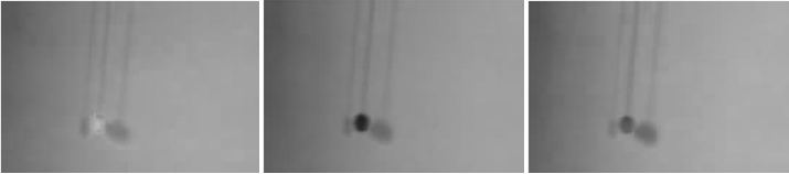
Figure 1. RGB layers of a single frame

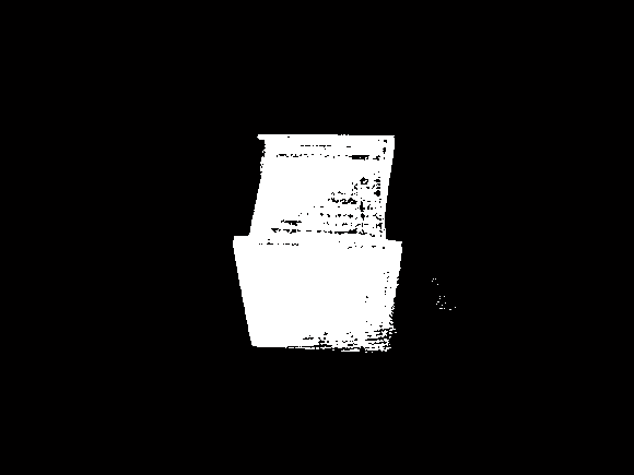
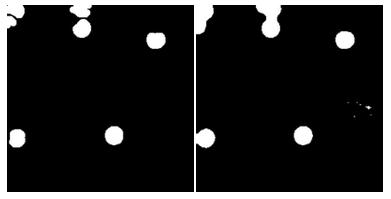
     The threshold value that was used was 0.5. Figure 2 shows the segmented image of five consecutive frames. Differences between consecutive frames are not very evident since there is 24.39 frames per second. 

Figure 2. Segmented images of five consecutive frames

     

     The method for obtaining the period and the acceleration due to gravity was quite unique. One way is to obtain the center of mass of the bob of the pendulum. However, an easier way is to observe the overlapping of consecutive frames.  The basic theory in a pendulum was utilized here. As the bob of the pendulum reaches the point of minimum kinetic energy, the distance travelled at a certain time decreases. Since the time interval between each frame is constant, the overlap between two consecutive frames increase. On the other hand, as the bob reaches the point wherein the kinetic energy is at its maximum the distance that the bob has move increases. Thus, the overlap between two consecutive frames is then smaller. 

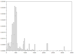
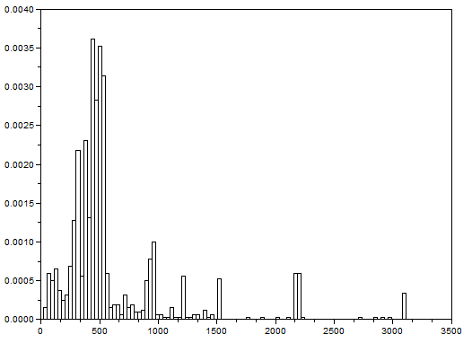
     To know the number of pixels that overlaps between consecutive frames, the images were first multiplied. Then the sum of the matrix of their product was obtained. This was done for 100 frames. Figure 3 shows the plot of the number of overlapping pixels vs. frame. It can be seen that there are several peaks. 

Figure 3. Number of overlapping pixels

     These peaks suggests the relative time at which the bob of the pendulum reaches minimum kinetic energy. Therefore, alternating peaks constitute for the period of the pendulum. Since there are 24.39 frames per second, the period of the pendulum is 1/24.39 which is equal to 0.0410004 sec. 

    Given the period and the length of the string, the acceleration due to gravity can then be calculated. Note that the length of the string is 30cm. From Figure 3, there are 26 frames that will complete a period. The acceleration due to gravity is given by

 
     Inserting all the obtained value for each parameters, the equation becomes

     The calculated acceleration due to gravity was found to be 10.409776m/sec. The analytical value for the acceleration due to gravity is 9.81m/sec. The percent error is then 

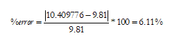
     The obtained percent error is relatively low. Thus, the use of image processing on series  of images to calculate physical quantities are also efficient. 

Reference

[1] Soriano, M. A12 - Video Processing. 2012



Self - evaluation

I will give myself a grade of 11 for producing the output in a more intuitive and a much easier manner. The calculated physical quantity was indeed near the accepted value. Also, ideas from previous activities were utilized. 

11th Activity: Color Image Segmentation

     Previously, regions of interest were isolated from their background. This is done to do more analysis and processing. Thresholding were done previously but this time, color will be used to segment images since thresholding won't be useful when grayscale value of the region of interest is the same as that of the background. 

     This activity will implement parametric and non-parametric probability distribution to segment images based on color. 

  

     For every pixel, there is a corresponding red, green, and blue values. The normalized chromaticity coordinates is given by

where I = R + G + B and r+g+b=1. Since b=1-r-g, the chromaticity can be explained by r and g. Figure 1 shows the normalized chromaticity space. 

Figure 1. The normalized chromaticity space

      An image of an object with a blue color was obtained as shown in Figure 2.  The blue box will then be segmented using the parametric and non-parametric probability distribution.  A monochromatic region was cropped from the region of interest. It is also shown in Figure 2. 

     

Figure 2. Image to be used for segmentation (left) ; patch from the image (right)

     The color of the patch was represented as points in the NCC space. Since the object is mainly blue, the coordinates must lie in the blue region in the NCC space. 

     After cropping a monochromatic part of the region of interest, the histogram of it was calculated. An algorithm was done in Scilab to derive the Gaussian Probability Distribution Function. The mean (μ_r and μ_g) and standard deviation (σ_r and σ_g) were first calculated. Then the probability can be obtained separately  by  

     This is then the probability that a certain pixel belongs to the region of interest. The joint probability is obtained by multiplying the probability that a pixel with chromaticity r to the probabilty that a pixel with chromaticity g belong to the ROI. 

     Figure 3 shows the resulting image after applying the Gaussian Probability Distribution Function. It can be seen that the

Figure 3. Output from parametric segmentation

        For the non-parametric probability distribution estimation, the location of the rg chromaticity was first taken and it is shown in Figure 4. The 2D histogram of the region of interest was obtained using the code provided in the manual: 

   

Figure 4. 2D histogram

     Figure 5 shows the resulting segmented image after histogram backprojection. The 2D histogram that was obtained previously was used to backproject the image to be segmented. 

Figure 5. Output from non-parametric segmentation

     It can be observed from the two methods were able to isolate the region of interest from its background. However, in the parametric segmentation the shading variations were more captured compared with the output from the non-parametric probability distribution estimation. The advantage of the non-parametric probability distribution estimation is that the use of histogram backprojection makes it a much easier method. 

     

Reference

[1] Soriano, M. A11 - Image Color Segmentation. 2010

Self-evaluation:

I would give myself a 10 for producing all the necessary output. I was also able to learn and understand the ideas behind the activity. 

Activity 10: Applications of Morphological Operations 3 of 3: Looping through Images

The final activity for the applications of morphological operations is about differentiating shapes with varying sizes in a given image. We will try to isolate the desired regions of interest from background noises.

Figure 1 is an image of circles which are actually punched papers. The whole image was divided into 99 sub-images with a size of 256x256 pixel. This was done automatically and randomly using Scilab.

Figure 1. Image of punched papers

     Figure 2 shows the sub-images. A sub-image was then opened and its histogram was also obtained to know the threshold value. It was found to be 0.8. Using this value, the sub-images were converted into binary sub-images as shown at the right in Figure 2.

Figure 2. Sub-images with 256x256 pixel each and their corresponding binarized sub-images

    The morphological operations such as open and close were used to clean the image. These are not readily available in SIP toolbox. However, these operations can be defined in terms of dilation and erosion operators. 

     Opening operator is the dilation of the eroded image with a same structuring element. It is given by 

where A is the image and B is the structuring element. 

     On the other hand, closing operator is the erosion of the dilated image. It is given by 

     Figure 3 shows the opening and closing of two sub-images. Indeed, the images were cleaned after applying opening and closing operations.

Figure 3. 1st column: original sub-images, 2nd column: Opening operator were applied; 3rd column: Closing operator were applied

      bwlabel  function was used to label each circle. The area of each circle for each sub-image was then calculated. Figure 4 shows the histogram of the area. It can be seen from the histogram that most of the blobs have an area from 450 to 600 pixels.

Figure 4. Histogram of area of blobs

       To obtain the best estimate, the area between the range of 450 to 600 pixels were averaged. Also the standard deviation was obtained. Thus, the area of the blob is 518.25±25.90 pixels. 

     The next task is to isolate the bigger cells shown in Figure 5. It was first turned to binary image with a threshold value of 0.8. 

Figure 5. Image of circles with enlarged circles

     A structuring element was created using a circle with a radius of 15pixels. The radius was such since we need to create a structuring element with an area slightly greater than the obtained area previously. Using morphological operations again, the bigger cells were then isolated from the background noise. Opening operator was used after it was eroded. The resulting image is shown in Figure 6.

Figure 6. Isolated enlarged blobs

References:

[1] Soriano, M. 2012. A10 Applications of Morphological Operations 3 of 3: Looping through Images

[2]en.wikipedia.org/wiki/Opening_(morphology)

[3]en.wikipedia.org/wiki/Closing_(morphology) 

Self-evaluation 

I would give myself a 10 since I was able to produce the necessary output and was able to explain my thoughts clearly. It was a very fun activity. :)

9th Activity: Applications of Morphological Operations 2 of 3: Playing Notes by Image Processing

     I was so surprised when I learned that Scilab could actually play notes! So before doing what was actually tasked to us, I first explored this function by playing some songs. :)  I have had piano lessons when I was a kid. I also had violin lessons at the Conservatory of Music. Aaaaand I love to sing. :) So as you could see, I really love music. So when asked to choose for a music sheet, I couldn't decide what to actually use after being familiar to lots of it.

     Going back to the real thing, I chose the first piece that I was able to play when I was a kid. It was entitled "Ode to Joy." The first line is shown in Figure 1.

Figure 1. First line of Ode to Joy

     I then inverted it and removed the g-clef as shown in Figure 2.

Figure 2. Inverted image

    Using the function imcorrcoef, the image is being compared to another image which is referred to as a template. I made a quarter note and a half note as templates as shown in Figure 3.

 

Figure 3. Templates to be used
  
     Thresholding was done after taking the result of the correlation. This was done to obtain a single pixel location for the quarter notes and half notes. These are shown in Figure 4 and Figure 5.

Figure 4. Locations of quarter notes

Figure 5. Location of half note

     Now that the locations of the notes are determined, the melody can now be played by assigning the frequencies for each note and then using the sound function. The sound file can now played below.



Reference
[1]Maricor Soriano. 2012. Activity 9 - Applications of Morphological Operations 2 of 3 - Playing Notes by Image Processing. Applied Physics 186

8th Activity: Applications of Morphological Operations1 of 3: Preprocessing Text

A scanned document was given to us as shown in Figure 1. Using the different morphological operations learned previously, handwritten texts will be extracted. 

Figure 1. Scanned document

     A part of the scanned document was scanned. Since the image was slightly tilted, it was corrected using GIMP. This correction is necessary for further steps to be done. The cropped image was converted to grayscale. These are shown Figure 2. 

 Figure 2. Cropped image and its grayscale format

     To remove the horizontal lines, a filter was applied. The Fourier transform of the image was first obtained. The filter was done by blocking the high frequencies in the Fourier transform.The FT of the image was then multiplied to the filter. Figure 3 shows the Fourier transform and the filter that was made (using GIMP).

Figure 3. Fourier transform of the cropped image and the filter used

    The resulting image is shown in Figure 4. It can be seen that the horizontal lines are now removed. However, the lines that intersected with the letters were also removed. Thus, the letters seems to be cut into half. :( Figure 5 shows the binarized image.

Figure 4. The resulting filtered image

   

Figure 5. Binarized image

     Dilation was applied to the image where the structuring element is a diagonal. I chose a diagonal as a structuring element to connect the letters since the handwriting is somewhat diagonally written. :) Figure 6 shows the resulting dilation.

Figure 6. Dilated image

     Since the image has become thicker, skel  was utilized to make it thinner. Figure 7 shows the resulting image.

Figure 7. Skeletonized(thinned) image

     It can be seen that some of the letter can be easily read now. :)


Reference:

[1] . Maricor Soriano, "A8 - Applications of Morphological Operations 1 of 3: Preprocessing Text", Applied Physics 186 Manual, 2012


Self-evaluation:
I admit I submitted this later due to SPP and my own research and experiments, but I would still give myself a 10. I was able to produce the necessary output and I was able to use concepts learned from previous activities.

7th Activity: Morphological Operations

This activity is about some morphological operations: erosion and dilation. We were tasked to hand-draw the effect of erosion and dilation on particular images. Predicted sketches were compared to the generated image from erode( ) and dilate( ) functions in Scilab. 

Erosion of an image A by structuring element B is denoted by 

where B_z   is the translation of B by z. The structuring element dictates the shape of the original image. It generally shrinks the size of the image. 

On the other hand, dilation is denoted by 

.

Dilation increases the shape of the original image according to the structuring element. 

To see the effects of erosion and dilation, different shapes were drawn and eroded by different structuring elements. Figure 1 shows the shapes that were drawn while Figure 2 shows the structuring elements used for each shape. 

Figure 1. Shapes to be eroded: square, triangle, hollow square, and plus sign

 Figure 2. Structuring elements: 2x2 ones, 2x1 ones, 1x2 ones, cross, diagonal 

Figure 3. Predicted effect of erosion(1st row) and dilation(2nd row) on a square

Figure 4.  Predicted effect of erosion(1st row) and dilation(2nd row) on a triangle 

Figure 5.  Predicted effect of erosion(1st row) and dilation(2nd row) on a hollow square 

Figure 6.  Predicted effect of erosion(1st row) and dilation(2nd row) on a plus sign 

     Lastly, the predicted images were compared to the output images generated by Scilab. Fortunately, the SIP toolbox has the functions erode( ) and dilate( ). It was quite easy then. Figure 7 to Figure 10 displays the output images when the shapes in Figure 1 were eroded and dilated by the structuring elements seen in Figure 2. 

Figure 7. Output images when square was eroded(1st row)
and dilated(2nd row) by the structuring elements

  

Figure 8. Output images when triangle was eroded(1st row)
and dilated(2nd row) by the structuring elements 

 

Figure 9. Output image when a hollow square was eroded(1st row)
and dilated(2nd row) by the structuring elements

Figure 10. Output image when plus sign was eroded(1st row)
and dilated(2nd row) by the structuring elements 

     

     It can be clearly seen that the predicted images matched the output images generated from Scilab. 

Reference:
[1] Soriano, M. A7 - Morphological Operations. 2012


Self-evaluation:

I will give myself a grade of 10/10 for understanding the concept of erosion and dilation. I was also able to present all the necessary output clearly.